I’ve been thinking about some ideas that climate blogger Willis Eschenbach (WE) has proposed. In particular, WE has suggested that tropical cumulus clouds and thunderstorms provide a “thermostatic mechanism” that helps to stabilize the temperature of the Earth within a narrow range. WE has also offered a procedure for predicting surface temperatures changes in response to increased radiative forcing.
I find both these ideas intriguing. Yet, there are assumptions implicit in WE’s thermostat hypothesis and predictive procedure—and I haven’t been at all certain that those assumptions are valid.
So, I wanted to do what I could to check those assumptions.
The Earth is a complex thermodynamic system. When it comes to understanding thermodynamic systems, my experience is that verbal reasoning often leads to incorrect conclusions. So, I always want to know what the what the math and physics tell us.
I’m not about to try to produce a complete, realistic model of Earth’s climate. However, I decided to apply math and physics to a simplified “toy model” of the Earth and its atmosphere.
Simplified models get some things right, and other things wrong. They’re not entirely trustworthy. Yet, such models can still offer valuable insights, beyond what one can get to with verbal reasoning alone.
With that in mind, I’ve analyzed a toy model I call “Thunderstorm World,” to see what light it could shed on WE’s procedure and hypothesis.
I’ve used this model to examine these questions:
- Does WE’s procedure for predicting how surface temperature changes in response to forcing seem likely to provide valid predictions?
- Does it seem likely that tropical cumulus clouds and thunderstorms might regulate the temperature of a planet to keep it within a narrow range?
Overview
This is a fairly long essay. So, I’ll offer an overview, and you can decide how much of the detailed exposition you want to read.
I describe the Thunderstorm World (TW) model, a simple model of a planet and its atmosphere which includes convective and radiative heat transfer and cloud-induced albedo changes.
The TW model exhibits strong convection and cloud formation at low latitudes. Among other results, the model yields a curve of surface temperature vs. total surface irradiance. This curve is qualitatively similar to the curve that emerges from measurements on Earth. This similarity offers a measure of validation for the model.
I apply a procedure proposed by Willis Eschenbach (or my understanding of that procedure) to trying to predict the response of the TW model to a “forcing” due to an increased concentration of greenhouse gases. Unfortunately, the procedure predicts an increase in mean global surface temperature that is too small by 45 percent. The procedure also fails to correctly predict the variation of temperature changes with latitude. I identify two mistaken assumptions implicit in the procedure that lead to these flawed predictions.
I examine whether tropical thunderstorms (or, more precisely, low-latitude convection and cloud formation) moderate or limit increases in planetary temperature. Within the TW model, it turns out that convection and cloud formation do moderate temperature increases. But these mechanisms don’t impose any hard limit on such increases. Although the onset of tropical convection might appear to act as a “thermostat” limiting surface temperature, in the TW model, the setting of this “thermostat” is relative to the temperature of the upper layer of the atmosphere. So, if a “forcing” warms the upper troposphere, then tropical surface temperatures can also rise.
Thus, to the extent that the TW model bears a relationship to real-world climate dynamics, the results of the model suggest that (a) the proposed procedure for predicting responses to forcing may not be trustworthy, and (b) tropical thunderstorms likely moderate but don’t place any absolute cap on planetary warming.
Table of Contents
- Overview
- The Thunderstorm World Model
- Basic TW Model Results
- Response to Greenhouse Gas Forcing
- Checking WE’s Procedure for Predicting Response to Forcing
- Why Doesn’t TICF Predict Temperature Correctly?
- Do Tropical Clouds and Convection Moderate Warming?
- Do Tropical Clouds and Convection Cap Warming?
- Relating the TW Model to Earth
- Conclusions
- APPENDIX: Model Details
The Thunderstorm World Model
The Thunderstorm World (TW) model is designed to be as simple as possible while still accounting for convective heat transfer, cloud formation, radiant heat transfer, and variations in surface temperature.
To this end, the TW model assumes:
- The planet has a uniform surface, high thermal inertia, rotates rapidly, and has no inclination, so that diurnal and seasonal temperature variations can be ignored, and there is no variation with longitude. Temperatures and energy flows depend only on the latitude, 𝛳.
- The atmosphere has two layers. Each layer of the atmosphere is characterized by a single temperature at a given latitude.
- Although the surface temperature, T₁(𝛳), and the temperature of the lower layer of the atmosphere, T₂(𝛳), vary with latitude, the temperature of the upper layer of the atmosphere, T₃, is the same at all latitudes. (On Earth, the average temperature in the upper troposphere at a pressure of 190 mbar is only weakly dependent on latitude, so this assumption of constant temperature isn’t unreasonable.)
- Convection happens whenever the temperature difference between the surface and the lower atmosphere layer, or between the lower and upper atmosphere layers, exceeds a threshold value 𝚪H, where 𝚪 is the adiabatic lapse rate and H is the elevation change between layers.
- The heat transfer rate associated with convection is assumed to be proportional to how much the temperature difference exceeds 𝚪H.
- When convection occurs at the surface, this is assumed to lead to cloud formation which leads to reflection of shortwave radiation from the Sun. This increase in albedo is assumed to be proportional to how much the temperature difference exceeds 𝚪H.
- The layers of the atmosphere have radiative properties similar to those assumed in my prior essay, Atmospheric Energy Recirculation. Each layer of the atmosphere absorbs fully a fraction f of thermal radiation wavelengths, and is transparent to a fraction (1– f) of thermal radiation wavelengths. The parameter f is taken to relate to the concentration of greenhouse gases present in the atmosphere.
- At a given latitude, the surface and the lower layer of the atmosphere are assumed to adjust their temperatures to ensure energy balance, so that the rate of energy entering and leaving match. For the upper layer of the atmosphere, energy balance is also assumed, but this requires integrating energy gained and lost over all latitudes, since air circulation is taken to maintain a uniform temperature for the upper layer of the atmosphere.
- Heat transfer between latitudes via atmospheric circulation is not fully modeled, but is addressed partially via the assumption that the temperature of the upper atmosphere is independent of latitude.
These assumptions vastly oversimplify the way Earth’s climate works. Yet, they include enough elements, and enough thermal physics, that perhaps some dynamics of the real system will be reproduced by the model.
The model is depicted below.

The surface receives energy from the Sun, more at the equator and less at the poles, and exchanges energy with the lower layer of the atmosphere, as well as radiating some energy directly to space. The lower and upper layers of the atmosphere also exchange energy, and the upper layer radiates energy to space.
At low latitudes (near the equator), surface heating leads to the adiabatic lapse rate being exceeded in a way that triggers convection.
In general, the zone where convection happens between the layers of the atmosphere may be different than the zone where convection happens between the surface and the lower layer of the atmosphere. (In a more complex variant of the TW model, these zones are more similar.)
That’s the TW model.
In what follows, I offer results for the dynamics of the model, based on model parameters as specified in the Appendix. Given those parameter values, I’ve numerically solved for the temperatures T₁(𝛳), T₂(𝛳), and T₃ and the energy flows that yield energy balance in steady-state.
Basic TW Model Results
For the model parameters I’ve considered, within the TW model temperatures vary with latitude as shown in the following figure.
Please keep in mind that I’m not expecting the TW model to accurately model Earth in any quantitative way. I’m just hoping to see some general qualitative similarities between dynamics of the model and some of the dynamics on Earth.

The figure shows how surface temperature (red curve) and the temperatures of the two layers of the atmosphere (green and blue curves) vary with latitude.
The surface temperature (red curve) rises as one moves from the polar region towards lower latitudes, until a latitude of 42º where a threshold temperature of 25.4℃ is achieved. After that threshold point, the surface temperature rises only very slowly, reaching 26.9℃ at the equator.
The surface temperature is very cold (-80℃) at the poles. This is because the TW model does not account for the air and ocean currents which warm Earth’s polar regions.
Averaging the surface temperature over the globe, the average surface temperature is 19.3℃, a little warmer than Earth. (In computing the average, latitudes nearer the equator are weighted more heavily than latitudes nearer the poles, because the surface has more area at lower latitudes.)
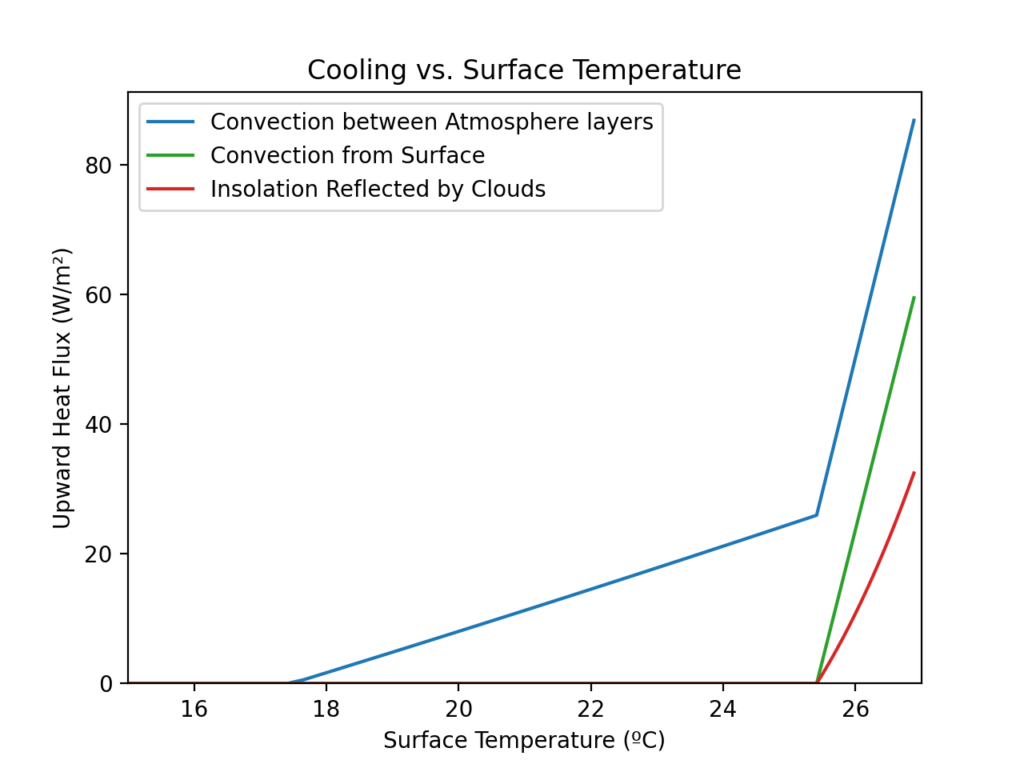
To understand why the temperature plot looks as it does, it helps to look at convective cooling effects, as shown below.

For latitudes below 52º, convection transports heat between the two layers of the atmosphere. For latitudes below 42º, surface convection transports heat into the atmosphere and forms clouds that reflect some of the incident shortwave radiation.
The onset of convection explains why the curve for surface temperature (in Figure 1) changes slope at these two threshold latitudes.
(On Earth, the threshold latitudes for the onset of major convection and ocean thunderstorms are closer to the equator than they are in the TW model for the parameters I’ve chosen. The oversimplifications in the TW model mean that one can choose only a few of Earth’s parameters to fit properly. I chose to roughly fit the insolation and mean surface temperature values for Earth, at the expense of allowing the threshold latitude to be significantly different than what is observed on Earth. I think this is ok, because I am interested in the qualitative behavior of the model, not the absolute value of any quantitative results.)
These cooling effects can also be plotted as a function of surface temperature, as shown below.
One can see that surface cooling increases rapidly for surface temperatures above 25.4℃. This seems qualitatively similar to what one sees in WE’s Figure 3. This offers reassurance that the TW model is reproducing some of the climate features that WE’s analysis relies upon.
Let’s look at another type of graph that WE uses.

This chart shows surface temperature as a function of total downwelling irradiance at the surface within the TW model. It is notable that the slope of the curve greatly flattens for irradiance values above about 450 W/m². This looks qualitatively quite similar to WE’s Figure 2, though the specific irradiance threshold value is different for the TW model and for the Earth.
In Figure 5, temperature increases monotonically with irradiance. This matches WE’s Figure 3 for land-based data, but differs from WE’s Figure 4 for ocean-based data. In the latter figure, temperature above the threshold declines somewhat with increasing surface irradiance.
Can the TW model account for such non-monotonic behavior?
It turns out that a variant of the TW model exhibits such behavior.

The simple form of the TW model uses the same adiabatic lapse rate, 𝚪, everywhere. In reality, the adiabatic lapse rate depends on the extent to which water vapor is present. For moist air, the lapse rate is smaller, and for dry air it is larger.
I would expect that the atmosphere is likely to be more humid where surface convection (presumed to be above an ocean) is happening, and less humid where there is no surface convection. So, the lapse rate for convection between the layers of the atmosphere ought to be larger when there is no surface convection, and smaller when there is surface convection. That’s the assumption used in the variant of the TW model that yields the temperature vs. irradiance curve in Figure 6.
In Figure 6, the temperature for a given irradiance drops as surface convection begins. This is qualitatively similar to what is observed in WE’s data for ocean locations.
Once again, I feel reassured that the predictions of the TW model qualitatively reproduce what WE has seen in data for Earth.
For the remainder of this essay, I’ll stick to the version of the TW model that yielded Figure 5, since that model is easier to understand.
Response to Greenhouse Gas Forcing
What does the TW model predict will happen if the concentration of greenhouse gases is increased?
Let’s consider a top-of-atmosphere (TOA) radiative forcing ∆F = 7.4 W/m², which I understand to be roughly the radiative forcing predicted to occur on Earth if the concentration of CO₂ was quadrupled.
As I understand climatologists’ use of the term, radiative forcing is a measure of the radiative imbalance that would occur at TOA if greenhouse gas concentrations were increased, but the atmosphere and surface were otherwise unchanged thermodynamically. I assume this means that all temperatures remain the same, as do convection and cloud coverage.
Based on this understanding, a TOA imbalance of 7.4 W/m² occurs in the TW model if the longwave absorption fraction, f, is increased from f = 0.600 to f = 0.631. So, to compute the effect of a TOA forcing ∆F = 7.4 W/m², I re-ran the TW model for f = 0.631, solving for the new temperatures, convective heat flows and cloud-induced albedo increases.
The old and new temperatures are shown below.

The mean global surface temperature in the TW model increases by 1.84℃.
Please don’t attach significance to this particular value. I don’t believe the absolute magnitude of this number to be meaningful, given the limitations of the TW model. What is likely to be meaningful, however, is how this value compares to other predictions of temperature change associated with the same model.
Checking WE’s Procedure for Predicting Response to Forcing
As I understand it, WE’s procedure for computing the Surface Response to Increased Forcing goes like this:
- For a given TOA radiative forcing value ∆Fₜ, compute an equivalent increase in downwelling surface irradiance, ∆Fₛ. In WE’s example, on Earth, a TOA forcing of ∆Fₜ=3.7 W/m² was thought to lead to a downwelling forcing 1.3 times as large (presumably leading to a ∆Fₛ=4.8 W/m² increase in downwelling radiation).
- Given a graph of surface temperature T₁ versus surface irradiance Eₑ, compute the derivative dT₁/dEₑ. (That graph might be WE’s Figure 3 or 4 or my Figure 5 or 6.)
- At each point on the planetary surface, compute the temperature change ∆T₁ as ∆T₁ = ∆Fₛ × (dT₁/dEₑ).
Let’s call this procedure Temperature-Irradiance Curve Following, or TICF. TICF might or might not be an accurate representation of the procedure that WE is advocating. He can let us know. Regardless, we can evaluate how well TICF works with respect to the TW model.
With regard to step #1 above, comparing the mean total (SW+LW) surface irradiance before and after applying the ∆Fₜ=7.4 W/m² TOA forcing (i.e., before and after increasing f from 0.600 to 0.631), the mean total surface irradiance ⟨Eₑ⟩ increases by ∆Fₛ=12.15 W/m². (So, in this case ∆Fₛ=1.6 × ∆Fₜ.)
When I apply step #2 to my Figure 5, then apply step #3 using ∆Fₛ=12.15 W/m², and average over the surface of the planet, the TICF procedure predicts a mean global surface temperature change of 1.02℃. That’s 45 percent less than the “actual” mean temperature change value of 1.84℃ produced by the TW model.
So, the TICF procedure did not do a very good job of predicting temperature changes in the TW model.
Why Doesn’t TICF Predict Temperature Correctly?
The TICF procedure is appealing intuitively. So, why doesn’t it correctly predict temperature changes?
As far as I can tell, there are two ways in which the TICF procedure as I outlined it goes wrong.
One problem with TICF, as I’ve outlined it, is that the surface irradiance forcing ∆Fₛ is assumed to be a constant that is independent of latitude.
Let’s look at how the surface irradiance changes when the forcing is applied (i.e., when f =0.600 changes to f =0.631).

The red curve (∆ SW+LW) indicates the change in total irradiance absorbed by the surface, ∆𝚽. As one can see, this is nowhere near being a constant. It depends strongly on latitude, 𝛳.
Let’s assume we know ∆Eₑ(𝛳), and try using this to predict temperature changes via the formula ∆T₁ = ∆Eₑ(𝛳) × (dT₁/dEₑ). We could call this procedure Spatially-Varied-Forcing TICF, or SVF-TICF. (This procedure isn’t likely to very useful in practice, even if it works, because anyone who knows ∆Eₑ(𝛳) probably also already knows the temperature change.)
How well does SVF-TICF predict temperature changes?

The chart above shows the change in surface temperature, as a function of latitude, as predicted by TICF, as predicted by SVF-TICF, and as in the actual solution of the TW model.
It’s apparent that the TICF procedure which assumes a constant forcing ∆Fₛ (green curve) matches the right answer (red curve) almost nowhere. It’s no wonder that its prediction of the change in mean surface temperature is way off.
What about SVF-TICF? For latitudes between 90º and 44º, the SVF-TICF predicted temperature change (blue curve) closely tracks the “Actual” temperature change within the TW model (red curve). So, that’s an improvement.
However, while it might be a little difficult to see in the chart, for latitudes between 44º and 0º, the TICF (green curve) and SVF-TICF (blue curve) predictions join together, and both predict tropical surface temperature increases much smaller than the “Actual” result (red curve).
Because a global average weights low latitudes strongly, the mean global surface temperature increase predicted by SVF-TICF is 1.05℃, just barely larger than the 1.02℃ predicted by TICF, and still much less than the actual increase of 1.84℃.
So, even with accurate information about spatial variations in the downwelling irradiance forcing, the SVF-TICF procedure fails to accurately predict temperature changes.
What is the core problem with TICF?
TICF depends on the assumption that the curve of surface temperature vs. surface irradiance is fixed, and that a “forcing” will simply cause different locations on the surface to change where they appear on this fixed curve.
So, the procedure is critically dependent on the temperature vs. irradiance curve not changing.
Unfortunately, the curve does change.

As seen in the chart above, the curve of surface temperature vs. total surface irradiance superficially looks mostly the same before and after the forcing is applied. But what is going on to the upper right? Let’s look at that part more closely.

Once total surface irradiance exceeds 450 W/m², the “initial” and “final” curves are different. Unfortunately, this region of the graph applies to a majority of the surface area of the planet.
If a forcing raises the temperature of the upper atmosphere layer (as can be seen to happen in Figure 7), this increases the temperature at which tropical thunderstorms “cap” the surface temperature. This is what shifts the temperature vs. irradiance curve.
To generalize this result a bit, the temperature vs. irradiance curve in the TW model is unchanged by forcing in locations where energy transfer is entirely radiative, but the curve changes in locations where convection is important.
Since convection and atmospheric circulation are important, albeit to varying degrees, almost everywhere on Earth, it seems likely that the temperature vs. irradiance curve on Earth might shift in response to forcing.
Thus, the TICF procedure seems unlikely to be effective in accurately predicting surface temperature changes in response to forcing.
Do Tropical Clouds and Convection Moderate Warming?
WE has suggested that tropical cumulus cloud formation and thunderstorms (supporting strong convective heat flows) help to moderate Earth’s temperature.
Let’s see what the TW model has to say about this hypothesis.
I redid the temperature change calculation, holding some factors fixed. Once again, I assumed a 7.4 W/m² TOA forcing, modeled by increasing the longwave absorption fraction from f=0.600 to f=0.631. The results for the increase in mean global surface temperature were:
- 2.61℃: cloud albedo and convective heat transfer held fixed.
- 2.05℃: cloud albedo held fixed and convective heat transfer allowed to adjust.
- 1.84℃: cloud albedo and convective heat transfer both allowed to adjust.
So, if a researcher failed to account for increased cloud albedo, they would predict a temperature change 11 percent larger than what actually happens in the TW model. If a researcher failed to account for both increased cloud albedo and increased convection, they would predict a temperature change 42 percent larger than what actually happens.
(I have the impression that the GCM computer codes used by climatologists all model convection changes. Some reading suggests that GCM’s typically also model cloud formation. But, I’m not an expert on GCM’s and would rather not get into a debate about them. Let’s stick to talking about what the TW model tells us.)
(The TW model likely overestimates the cooling effect of clouds because the model accounts for increased reflection of sunlight from clouds, but does not account for increased longwave absorption and emission from clouds, which tend to have a warming effect. On Earth, on average, longwave warming by clouds compensates for about 60 percent of the shortwave cooling by clouds, although cooling effects predominate more strongly in the tropics, as indicated by WE Figure 2.)
The bottom line is that the hypothesis that “increases in tropical cloud formation and convection moderate planetary warming” is valid within the TW model.
Do Tropical Clouds and Convection Cap Warming?
The results of the TW model do not support the hypothesis that “tropical cloud formation and thunderstorms place a hard limit on planetary temperature increases.”
In the TW model, there is not an absolute “thermostat” effect that prevents tropical surface temperatures from increasing in response to a forcing. To the contrary, the temperature at the equator increased by 1.46℃ in response to the forcing.
What may be confusing is that there is a relative “thermostat” effect that prevents tropical surface temperatures from increasing too much, within the context of a given upper atmosphere layer temperature.
So, in the context of the baseline TW model, surface convection is triggered at a surface temperature of 25.4℃ at a latitude of 42º, and once convection is active temperature increases slowly to a maximum of 26.9℃ at the equator.
This might make it appear that there is a “thermostat” set at 25.4℃.
However, after the forcing is applied, surface convection is triggered at a surface temperature of 26.8℃ at a latitude of 43º, and once convection is active temperature increases slowly to a maximum of 28.3℃ at the equator.
So, there still appears to be a “thermostat”, but after the forcing, the thermostat is set 1.4℃ higher.
The reason it works this way is that the onset of surface convection is governed by the lapse rate and the temperature of the upper layer of the atmosphere. The forcing caused the temperature of the upper layer of the atmosphere to increase by 1.4℃. In the TW model, this leads to a corresponding increase in the “maximum surface temperature” in low latitudes.
The lesson to be learned from this is that, within the TW model, tropical thunderstorms cap the maximum surface temperature, but only relative to the temperature of the upper atmosphere layer. If the temperature of the upper atmosphere layer (i.e., the upper troposphere) increases as a result of forcing, then the temperature limit enforced by tropical thunderstorms will increase as well.
Relating the TW Model to Earth
How does the TW model relate to Earth?
The TW model certainly leaves out many processes which are important in Earth’s climate. Earth’s atmosphere includes many layers, and is affected by global circulation patterns in the atmosphere and oceans, circulation patterns which are largely unaccounted for in the TW model. The radiative dynamics in Earth’s atmosphere are also more complex than those assumed in the TW model.
The parameters used in the TW model example I’ve presented lead to behavior that matches Earth in some ways (e.g., insolation and global temperature are at least vaguely comparable in the TW example and on Earth) but not in others (e.g., strong convection occurs over a broader range of latitudes in the TW example than on Earth). The simplifications in the TW model mean that its behavior can’t be quantitatively matched to that of Earth except in a few respects.
Yet, the TW model includes the dynamics of the onset of convection in a way that seems likely to be at least somewhat relevant to the way things work on Earth. Both in the TW model and on Earth, convection is stimulated when surface warming causes the adiabatic lapse rate to be exceeded. This creates a threshold effect that is relative to the temperature of the upper troposphere.
I think the TW model is accurate in portraying this aspect of climate physics.
Conclusions
Based on working with the Thunderstorm World model, it seems to me that:
- It makes sense to be skeptical about the ability of the TICF procedure to accurately predict how surface temperatures would respond to forcing.
- Tropical cumulus clouds and convection associated with thunderstorms likely moderate planetary temperature changes, but aren’t likely to provide any fixed limit on planetary warming.
APPENDIX: Model Details
At a given latitude, 𝜽, the net energy flows within the Thunderstorm World (TW) model are as depicted in the following illustration.

For the calculations presented in this essay, the following parameter values were used:
- Mean insolation, Sₐ = 292.6 W/m². (This is approximately the insolation Earth experiences, if non-cloud albedo is taken into account.)
- Convection adiabatic lapse threshold, 𝚪H = 30 Kelvin.
- Convection strength, Z = 0.2 /Kelvin.
- Convection heat flux reference value, Sᵣ = Sₐ. (To apply a “forcing” associated with increased insolation, one should increase Sₐ without increasing Sᵣ.)
- Convection heat-transfer vs. cloud-formation fraction, 𝝌 = 0.7.
- Long-wave radiation absorption fraction, f = 0.6 (prior to added forcing).
The area-weighted global average of a quantity g(𝜽) is given by the integral from −𝜋/2 to 𝜋/2 of ½⋅cos(𝜽)⋅g(𝜽).
For the variable-water-vapor model variant used to generate Figure 6, the adiabatic lapse threshold 𝚪₂H for convection between the lower and upper atmosphere layers is made to transition from 33 K to 30 K as surface convection begins. (In particular, this transition is made as the value of T₁’ − T₂’ − 𝚪₁H transitions from -1 K to 1 K, where T₁’ and T₂’ are the values that T₁ and T₂ would have if only radiative heat flows were present, and where 𝚪₁H = 30 K. This somewhat peculiar recipe was chosen because it was found to support numerical convergence.)